
Summary
Science Score had a mean of 51.85 (SD = 9.90). Math Score had a mean of
52.65 (SD = 9.37). Read Score had a
mean of 52.23 (SD = 10.25). Further,
shape of histograms together box-plots suggested an approximate normal
distribution for all these variables.
Among
200, 84% of schools were of Public type and 16% of schools were of Private
type. In Types of Programs, 22.5% had general program, 52.50% had academic
programs and 25% had vocational programs. There was a significant association
prevailing between Types of programs and Types of schools.
Math
and reading scores had highest coefficient of correlation in the tune of 0.662.
The prediction equation thrown by regression analyis was , Science score = 16.76 + 0.667*Math score.
Overall the model was found fit as the F-statistics
was significant with a p-value as
0.000. Math score was able to explain approximately 40% of total variance in
science score.
Social
Studies scores had mean 52.405 and standard deviation as 10.736. There were 109
females and 91 males out of total of 200 cases. 147 cases had shown writing
score less than 60, whereas 53 cases had scored equal to more than 60. Low,
middle and high categories of ses were 47, 95 and 58 respectively.
The
prediction equation for predicting Science scores thrown by multiple linear
regression was: Science score = 12.325 +
0.389*math score + 0.05*social studies score + 0.335*reading score
-2.010*female. Predictors were able to
explain approximately 49% of total variance in science score. There was no linear relationship
between female and science score found through t-test. Confidence Interval for
regression coefficient of female were found between -4.0202 and 0.0002 at 95%
level.
Logistic
regression Model was found fit as Hosmer Lameshow Chi-square statistics was
found non-significant. The Logistic regression equation was found as: Honcomp = -10.201 + 0.098*read + 0.066*science
+ 0.110*ses. Overall classification accuracy was found as 78.51% with
91.80% for group-0 and 41.50% for group-1.
Other
than attsc4, first 5 items measuring attitude towards schools were found in
second factor. Factor analysis had thrown twelve factors. However, based on
scree plot, it is recommended that we should consider only three factors.
Factor loading tells us the relationship between individual items with their
corresponding factors. When only two factors were extracted, all ten items
measuring attitude towards school belonged to second factor. Internal
consistency of variables measuring attitude towards school was found ok.
Conclusions:
1. Science,
Math, Read, Write, Social studies were found approximately normal.
2. Significant
association between Types of programs and Types of schools was found through
Chi-square test.
3. The
coefficients of correlation between science, math and reading score were found
between 0.630 and 0.661.
4.
Scatter plot showed a
positive relationship between science and math scores.
5.
The
simple linear regression for predicting Science score with math score as independent
variable had R-square as 39.80%. The model was found fit.
6.
The
multiple linear regression for predicting Science score with math score, social
studies score, reading score and female as independent variables had R-square
as 48.90%. the model was found fit. Linear relationship between female and
science score was not confirmed by T-test.
7.
Overall classification
accuracy was found as 78.51% with 91.80% for group-0 and 41.50% for group-1
through Logistic regression model for predicting honcomp.
8. Based
on scree plot, we should consider only three factors. The internal consistency of
variables measuring attitude towards school was ok.
Recommendations
1. Science
score was better predicted by Multiple regression model hence should be used for
prediction.
2. Classification
accuracies were comparatively very low in group-0 against group-1, hence,
alternate models should be explored.
3. Analyst/researcher
should use the factor analysis results along with his past experience and
judgment for data reduction purpose.
3.1.1
Summary of science, math and read scores.
Descriptive
statistics has been shown in Table 3.1.1-1: Descriptives
and Histograms and Box plots are shown in Figure 3.1.1-1: Histograms and Box Plots.
Science Score had a mean of 51.85 (SD = 9.90). The median value was found
as 53.23 which was almost same as that of mean. Hence, mean can be considered
as a reasonable estimator of central tendency. Minimum and maximum values were
found as 26 and 74. Skewness and kurtosis values were found within +,- 2 and
shape of histogram together suggested an approximate normal distribution.
Further, box-plots had not shown any outliers.
Math Score had a mean of 52.65 (SD = 9.37). The median value was found as 52.00 which was almost
same as that of mean. Hence, mean can be considered as a reasonable estimator
of central tendency. Minimum and maximum values were found as 33 and 75. Skewness
and kurtosis values were found within +,- 2 and shape of histogram together
suggested an approximate normal distribution. Further, box-plots had not shown
any outliers.
Read Score had a mean of 52.23 (SD = 10.25). The median value was found as 50.00 which was almost
same as that of mean. Hence, mean can be considered as a reasonable estimator
of central tendency. Minimum and maximum values were found as 28 and 76.
Skewness and kurtosis values were found within +,- 2 and shape of histogram
together suggested an approximate normal distribution. Further, box-plots had
not shown any outliers.
Table
3.1.1-1
Descriptives
|
Descriptive Statistics
|
science
|
math
|
read
|
|
|
Mean
|
51.85
|
52.65
|
52.23
|
|
|
95% Confidence
Interval for Mean
|
Lower Bound
|
50.47
|
51.34
|
50.80
|
|
Upper Bound
|
53.23
|
53.95
|
53.66
|
|
|
5% Trimmed Mean
|
51.96
|
52.39
|
52.14
|
|
|
Median
|
53.00
|
52.00
|
50.00
|
|
|
Variance
|
98.03
|
87.77
|
105.12
|
|
|
Std. Deviation
|
9.90
|
9.37
|
10.25
|
|
|
Minimum
|
26.00
|
33.00
|
28.00
|
|
|
Maximum
|
74.00
|
75.00
|
76.00
|
|
|
Range
|
48.00
|
42.00
|
48.00
|
|
|
Interquartile Range
|
14.00
|
14.00
|
16.00
|
|
|
Skewness
|
-0.19
|
0.29
|
0.20
|
|
|
Kurtosis
|
-0.56
|
-0.65
|
-0.62
|
|
Figure
3.1.1-1
Histograms and Box
Plots
|
Variable↓
|
Histogram
|
Box plot
|
 3.1.2
(a) Table of type of school and type
of program.
3.1.2
(a) Table of type of school and type
of program.
Interpretation of Row and Column
percentages:
Screen shot 3.1.2-1: Cross tabulation shows percentages within each cells. Overall
Public schools were 84% and Private schools were 16%. Under types of program,
general. Academic and vocation were 22.50%, 52,50% and 25% respectively.
Within
Public type of schools, general were 19.50%, academic were 40.50% and vocation
were 24%. Within Private type of schools, general were 3%, academic were 12%
and vocation were only 1%.
Screen
shot 3.1.2-1
Cross tabulation

3.1.2
(b) Association between type of school
and type of program.
Hypotheses were designed as follows:

SPSS Output is shown in Screen shot 3.1.2-1 for Chi-square test. The chi-square statistics was found as 9.269 with 2 degrees of freedom and significance value was less than the level of significance, 5%. This indicated the rejection of null hypothesis and we can conclude that a significant association between both the types was existing. Further, the strength of association, as indicated by Phi was found as 0.215.
Screen shot 3.1.2-1:
Chi-square tests

3.1.3
Correlation between science, math and
read.
Screen shot 3.1.3: Correlations shows the SPSS output for bi-variate correlation
analysis. The maximum correlation was found between Math and Read in the tune
of 0.662 followed by Science and Math as 0.631. Almost the same correlation was
found between Science and Read as 0.630.
Screen shot 3.1.3:
Correlations

3.1.4
Scatter plot between science and math.
Screen shot 3.1.4: Scatter Plot shows the SPSS output for scatter plot between Science and Math scores. The trend line shows that there is a Positive
relationship existing between two variables. Further, the coefficient of
determination is 0.398 which shows that 39.80 percent of total variance in
Science score was explained by Math scores.
Screen shot 3.1.4:
Scatter
Plot

3.1.5
Simple Linear Regression between science
and math.
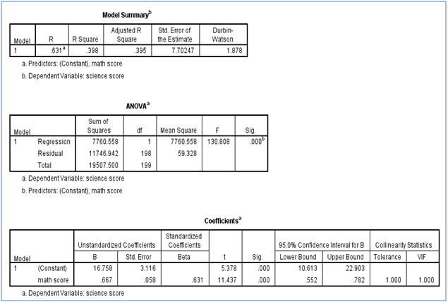
Screen
shot 3.1.5: Regression Output shows
the SPSS output for Simple Linear Regression between Science (Response Variable) and Math
scores (Explanatory Variable).
The
relationship between Science and Math scores were found positive as indicated
by the positive sign of regression coefficient 0.667. The linearity of
relationship was further supported by the significance value of regression
coefficient. It was found less than
0.05. The coefficient of correlation was indicated a 0.631 which was same as
found in previous analysis under section 3.1.3. R-square value was found as
0.395 which was reflected in scatter plot also.
The
Durbin Watson Statistics was 1.878 which showed that there was no
autocorrelation. Overall model was found good as F-statistics was significant
(p-value was <.= 0.01). Standard Error of estimate was found as 7.702.
Screen shot 3.1.5:
Regression
Output
3.2
Descriptive Analysis
As I have
already presented the Descriptive Analysis for science, math and read under
3.1.1, I am presenting for Descriptive Analysis for socst, female, honcomp and ses under the following section.
Variable: Social Studies Score (socst)
Social Studies Score had a mean of 52.405 (SD = 10.736). The median value was found
as 52.41 which was almost same as that of mean. Hence, mean can be considered
as a reasonable estimator of central tendency. Minimum and maximum values were
found as 45 and 71. Descriptive statistics is shown in Screen shot 3.2-1.
Skewness and kurtosis values were found within +,- 2
and shape of histogram together suggested an approximate normal distribution.
Further, box-plots had not shown any outliers as shown in Figure 3.2-1.
Screen
shot 3.2-1
Descriptive Statistics
of Social Studies Score (socst)

Figure
3.2-1
Histogram & Box
Plot of Social Studies Score

Variable: Female, honcomp and ses
The
frequencies of female, honcomp and ses were shown in Bar Diagrams in Figure
3.2-2. There were 91 males and 109 female respondents. 53 respondents have
scored more than or equal to 60 in writing score. Rest 147 scored less than 60
in writing score. There were 47, 95 and 58 respondents under low, middle and
high categories of ses variable.
Figure
3.2-2
Bar Diagrams of female,
honcomp and ses

3.2.1
(a) Regression Equation and Output
The regression equation found is as follows:
 Regression output is shown in Screen
shots 3.2-2 and 3.2-3.
Regression output is shown in Screen
shots 3.2-2 and 3.2-3.
Screen
shot 3.2-2
Regression Output-Coefficients

Screen
shot 3.2-3
Regression Output-Model
Summary and ANOVA results
For Complete Assignment, send us a mail to info@sampleassignment.com
We do not just offer research paper
services. We have other services including writing dissertations, book reports,
editing and proofreading, lab reports and admission essays among others. Our
team of experts at Sample Assignment have
high degrees including MA’s and PHD’s. We guarantee you a 100% plagiarism free
original research papers. Our papers are well written, free from grammatical
mistakes and come at competitive prices that fits your needs. Buy research papers from Sample Assignment now!
No comments:
Post a Comment